利用 ERA5 数据驱动 WRF-chem

jokervTv 2021/11/21

数据下载
WPS
- vim namelist.wps
  - shared
  - geogrid
  - ungrib
  - metgrid
- run
WRF
- vim namelist.input
- run
  - real
  - wrf.exe
参考

# 数据下载

3D Data (e.g. data on pressure levels)

Temperature ('temperature')
U and V components of Wind ('u_component_of_wind','v_component_of_wind')
Geopotential Height ('geopotential')
Relative Humidity (the code can calculate RH if Specific Humidity is available;this is controlled in the Vtable) ('relative_humidity','specific_humidity')

2D Data (e.g. data on single levels)

# WPS

由于原 WPS 和 WRF 目录下文件太乱，所以个人比较喜欢到单独的地方运行，需要如下准备

mkdir   wps_case_data
cd      wps_case_data

ln -s   $WPS_DIR/geogrid.exe
ln -s   $WPS_DIR/ungrib.exe
ln -s   $WPS_DIR/metgrid.exe
cp      $WPS_DIR/link_grib.csh ./
cp      $WPS_DIR/namelist.wps ./

1
2
3
4
5
6
7
8

# vim namelist.wps

根据用户手册 (opens new window) 修改各个选项即可

# shared

PS：由于 geogrid 仅生成与时间无关的数据，因此 geogrid 会忽略 start_date、end_date 和 interval_seconds 变量。

# geogrid

在 &geogrid 部分，定义了模拟域的投影，以及所有模型网格的大小和位置。用于模型域的地图投影由 map_proj 变量指定。 ARW 中四种可能的地图投影中的每一种都在下面的整页图中以图形方式显示，用于设置投影参数的名称列表变量总结在下表中

Map projection / value of map_proj	Projection parameters
Lambert Conformal / 'lambert'	truelat1
	truelat2 (optional)
	stand_lon

Mercator / 'mercator'	truelat1

Polar stereographic / 'polar'	truelat1
	stand_lon

Regular latitude-longitude, or cylindrical	pole_lat
equidistant / 'lat-lon'	pole_lon
	stand_lon

个人喜欢添加

 OPT_GEOGRID_TBL_PATH = './'

# ungrib

none

# metgrid

个人喜欢添加

 OPT_METGRID_TBL_PATH = './'

# run

# geogrid.exe

选择合适的 TBL，由于我运行的是 WRF-CHEM，故选择 GEOGRID.TBL.ARW_CHEM

ln -s $WPS_DIR/geogrid/GEOGRID.TBL.ARW_CHEM GEOGRID.TBL

运行

./geogrid.exe

然后查看运行提示，如有错误，按照提示解决即可。例如 Could not open /opt/app/wrf/WPS_GEOG/soiltype_top_5m/index

则到官方网站 (opens new window) 下载对应文件都行。

完成后有如下提示：

!!!!!!!!!!!!!!!!!!!!!!!!!!!!!!!!!!!!!!!!!!!!!
!  Successful completion of geogrid.        !
!!!!!!!!!!!!!!!!!!!!!!!!!!!!!!!!!!!!!!!!!!!!!

1
2
3

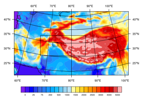
显示地理位置区域，简单修改官网实例文件如下，可校验区域是否按预期设置：
（相对于 WPS 自带的区域绘制图，叠加了地形）

; Overlay information from 2 domains
; November 2009

load "$NCARG_ROOT/lib/ncarg/nclscripts/csm/gsn_code.ncl"
load "$NCARG_ROOT/lib/ncarg/nclscripts/csm/gsn_csm.ncl"
load "$NCARG_ROOT/lib/ncarg/nclscripts/wrf/WRFUserARW.ncl"

begin

  wks = gsn_open_wks("pdf", "wrf_overlay_doms")  ; Open graphics file

  d1 = addfile("./geo_em.d01.nc", "r")
  d2 = addfile("./geo_em.d02.nc", "r")
  d3 = addfile("./geo_em.d03.nc", "r")


  var1 = wrf_user_getvar(d1,"HGT_M",0)
  lat1 = wrf_user_getvar(d1,"XLAT",0)
  lon1 = wrf_user_getvar(d1,"XLONG",0)
  var2 = wrf_user_getvar(d2,"HGT_M",0)
  lat2 = wrf_user_getvar(d2,"XLAT",0)
  lon2 = wrf_user_getvar(d2,"XLONG",0)
  var3 = wrf_user_getvar(d3,"HGT_M",0)
  lat3 = wrf_user_getvar(d3,"XLAT",0)
  lon3 = wrf_user_getvar(d3,"XLONG",0)

  var1@lat2d = lat1
  var1@lon2d = lon1
  var2@lat2d = lat2
  var2@lon2d = lon2
  var3@lat2d = lat3
  var3@lon2d = lon3

  dom_dims = dimsizes(var1)
  dom_rank = dimsizes(dom_dims)
  nx1 = dom_dims(dom_rank - 1) - 1
  ny1 = dom_dims(dom_rank - 2) - 1
  dom_dims = dimsizes(var2)
  dom_rank = dimsizes(dom_dims)
  nx2 = dom_dims(dom_rank - 1) - 1
  ny2 = dom_dims(dom_rank - 2) - 1
  dom_dims = dimsizes(var3)
  dom_rank = dimsizes(dom_dims)
  nx3 = dom_dims(dom_rank - 1) - 1
  ny3 = dom_dims(dom_rank - 2) - 1

  res                 = True

; Set some contouring resources.
  res@cnFillOn        = True
  res@cnLinesOn       = False
  res@cnLineLabelsOn  = False
  res@cnInfoLabelOn   = False
  res@gsnSpreadColors = True
  res@cnLevelSelectionMode = "ExplicitLevels"
  res@cnLevels             = (/0, 10, 25, 50, 75, 125, 200, 350, 500, 750, \
                                1000, 1250, 1500, 1750, 2000, 2250, 2500, 2750, 3000, 3500, 4000, 4500, 5000/)
  res@gsnLeftString = ""
  res@gsnRightString = ""

  res@gsnDraw         = False
  res@gsnFrame        = False

  res2 = res
  res3 = res
; Add map resources
  res@mpDataBaseVersion     = "MediumRes"          ; Default is LowRes
  res@mpOutlineDrawOrder    = "PostDraw"           ; Draw map outlines last
  res@mpGridAndLimbOn       = True                 ; Turn off lat/lon lines
  res@mpGridLonSpacingF     = 10
  res@mpGridLatSpacingF     = 5
  res@gsnMajorLatSpacing    = 5
  res@gsnMajorLonSpacing    = 10
  res@pmTickMarkDisplayMode = "Always"             ; Turn on map tickmarks
  res = set_mp_wrf_map_resources(d1,res)
  res@mpLimitMode        = "Corners"               ; Portion of map to zoom
  res@mpLeftCornerLatF   = lat1(0,0)
  res@mpLeftCornerLonF   = lon1(0,0)
  res@mpRightCornerLatF  = lat1(ny1,nx1)
  res@mpRightCornerLonF  = lon1(ny1,nx1)

; Add label bar resources
  res@lbLabelAutoStride = True
  res@gsnMaximize     = True    ; Maximize plot in frame


  res2@lbLabelBarOn = False  ; Labelbar already created in 1st plot
  res2@gsnMaximize  = False  ; Use maximization from original plot

  res3@lbLabelBarOn = False  ; Labelbar already created in 1st plot
  res3@gsnMaximize  = False  ; Use maximization from original plot

; we need these to later draw boxes for the location of the nest domain
  xbox_out = new(5,float)
  ybox_out = new(5,float)
  lnres = True
  lnres@gsLineThicknessF  = 1.5

; make images
  map = gsn_csm_contour_map(wks, var1, res)
  plot = gsn_csm_contour(wks, var2, res2)
  plot2 = gsn_csm_contour(wks, var3, res3)

; PLOT 3
  draw(map)   ; domain 2 already overlaid here - so just draw again
  xbox = (/lon2(0,0),lon2(0,nx2),lon2(ny2,nx2),lon2(ny2,0),lon2(0,0)/)
  ybox = (/lat2(0,0),lat2(0,nx2),lat2(ny2,nx2),lat2(ny2,0),lat2(0,0)/)
  datatondc(map, xbox, ybox, xbox_out, ybox_out)
  gsn_polyline_ndc(wks, xbox_out, ybox_out, lnres)

  xbox = (/lon3(0,0),lon3(0,nx3),lon3(ny3,nx3),lon3(ny3,0),lon3(0,0)/)
  ybox = (/lat3(0,0),lat3(0,nx3),lat3(ny3,nx3),lat3(ny3,0),lat3(0,0)/)
  datatondc(map, xbox, ybox, xbox_out, ybox_out)
  gsn_polyline_ndc(wks, xbox_out, ybox_out, lnres)

  frame(wks)

; print box point

  xbox1 = (/lon1(0,0),lon1(0,nx1),lon1(ny1,nx1),lon1(ny1,0)/)
  ybox1 = (/lat1(0,0),lat1(0,nx1),lat1(ny1,nx1),lat1(ny1,0)/)
  xbox2 = (/lon2(0,0),lon2(0,nx2),lon2(ny2,nx2),lon2(ny2,0)/)
  ybox2 = (/lat2(0,0),lat2(0,nx2),lat2(ny2,nx2),lat2(ny2,0)/)
  xbox3 = (/lon3(0,0),lon3(0,nx3),lon3(ny3,nx3),lon3(ny3,0)/)
  ybox3 = (/lat3(0,0),lat3(0,nx3),lat3(ny3,nx3),lat3(ny3,0)/)

  print("domains 1:")
  print(tostring(xbox1(1)) + " " + tostring(ybox1(1)) + " " + "-------" + tostring(xbox1(2)) + " " + tostring(ybox1(2)))
  print(tostring(xbox1(3)) + " " + tostring(ybox1(3)) + " " + "-------" + tostring(xbox1(0)) + " " + tostring(ybox1(0)))
  print("domains 2:")
  print(tostring(xbox2(1)) + " " + tostring(ybox2(1)) + " " + "-------" + tostring(xbox2(2)) + " " + tostring(ybox2(2)))
  print(tostring(xbox2(3)) + " " + tostring(ybox2(3)) + " " + "-------" + tostring(xbox2(0)) + " " + tostring(ybox2(0)))
  print("domains 3:")
  print(tostring(xbox3(1)) + " " + tostring(ybox3(1)) + " " + "-------" + tostring(xbox3(2)) + " " + tostring(ybox3(2)))
  print(tostring(xbox3(3)) + " " + tostring(ybox3(3)) + " " + "-------" + tostring(xbox3(0)) + " " + tostring(ybox3(0)))

end

1
2
3
4
5
6
7
8
9
10
11
12
13
14
15
16
17
18
19
20
21
22
23
24
25
26
27
28
29
30
31
32
33
34
35
36
37
38
39
40
41
42
43
44
45
46
47
48
49
50
51
52
53
54
55
56
57
58
59
60
61
62
63
64
65
66
67
68
69
70
71
72
73
74
75
76
77
78
79
80
81
82
83
84
85
86
87
88
89
90
91
92
93
94
95
96
97
98
99
100
101
102
103
104
105
106
107
108
109
110
111
112
113
114
115
116
117
118
119
120
121
122
123
124
125
126
127
128
129
130
131
132
133
134
135
136
137

# ungrib.exe

连接对应数据的变量表，这里使用 ERA5，故而对应 Vtable.ECMWF

ln -s $WPS_DIR/ungrib/Variable_Tables/Vtable.ECMWF Vtable

然后链接变量

link_grib.csh DATA_DIR/*

运行

./ungrib.exe

如下图所示即为成功

!!!!!!!!!!!!!!!!!!!!!!!!!!!!!!!!!!!!!!!
!  Successful completion of ungrib.   !
!!!!!!!!!!!!!!!!!!!!!!!!!!!!!!!!!!!!!!!

1
2
3

# metgrid.exe

连接对应的 METGRID.TBL.ARW

ln -s ./metgrid/METGRID.TBL.ARW METGRID.TBL

如果遇到以下错误

WARNING: Field PRES has missing values at level 200100 at (i,j)=(1,1)
WARNING: Field PRESSURE has missing values at level 200100 at (i,j)=(1,1)
WARNING: Field PMSL has missing values at level 200100 at (i,j)=(1,1)
WARNING: Field PSFC has missing values at level 200100 at (i,j)=(1,1)
WARNING: Field SOILHGT has missing values at level 200100 at (i,j)=(1,1)
ERROR: Missing values encountered in interpolated fields. Stopping.

1
2
3
4
5
6

这是因为在模拟域的范围内，气象数据缺失，通常是由于模拟域设置过大，调整 e_we 和 e_sn 到合适即可

# WRF

由于原 WPS 和 WRF 目录下文件太乱，所以个人比较喜欢到单独的地方运行，需要如下准备

mkdir   wrf_case_data
cd      wrf_case_data

ln -s   $WRF_DIR/run/real.exe
cp      $WRF_DIR/run/namelist.input ./

ln -s   $WRF_DIR/run/wrf.exe
ln -s   $WRF_DIR/run/*.TBL ./
ln -s   $WRF_DIR/run/ozone* ./
ln -s   $WRF_DIR/run/R* ./

1
2
3
4
5
6
7
8
9
10

# vim namelist.input

参考 README.namelist (opens new window) 一步步设置，还是有些头疼的

这里就省略了

# run

# real

ln -s ../wrf_case_data/met_em.d0* ./

./real.exe

如果看到了以下错误

forrtl: severe (174): SIGSEGV, segmentation fault occurred
Image              PC                Routine            Line        Source
real.exe           0000000002EB325A  for__signal_handl     Unknown  Unknown
libpthread-2.28.s  00007F28FF82CB20  Unknown               Unknown  Unknown
real.exe           0000000000468CD7  Unknown               Unknown  Unknown
real.exe           00000000004C2F48  Unknown               Unknown  Unknown
real.exe           00000000004CFEED  Unknown               Unknown  Unknown
real.exe           0000000000419E8C  Unknown               Unknown  Unknown
real.exe           0000000000418A22  Unknown               Unknown  Unknown
libc-2.28.so       00007F28FEAF2493  __libc_start_main     Unknown  Unknown
real.exe           000000000041892E  Unknown               Unknown  Unknown

1
2
3
4
5
6
7
8
9
10
11

可以尝试取消资源限制

ulimit -s unlimited

查看运行结果

cat ./rsl.error.0000

成功的话，最后一行如下

real_em: SUCCESS COMPLETE REAL_EM INIT

# wrf.exe

namelist.input 的时间逻辑我还没理清, 遇到如下错误

ERROR: Ran out of valid boundary conditions in file wrfbdy_d01

用

ncdump -v Times wrfbdy_d01

查看 wrfbdy_d01 时间维度，发现正好差一天，修改 namelist 即可，成功后

wrf: SUCCESS COMPLETE WRF

PS: 运行 wrf.exe 的时候依然遇到了 forrtl: severe (174): SIGSEGV, segmentation fault occurred，最后更换编译器解决，namelist.input 一模一样，我愿称其为玄学。

# 参考

https://dreambooker.site/2018/04/20/Initializing-the-WRF-model-with-ERA5/ (opens new window) http://bbs.06climate.com/forum.php?mod=viewthread&tid=40449 (opens new window)

jokervTv 爬坑历程

Choose mode